Neural Networks Specialist: Machine Learning Models Can Fail And Here Is Why

We usually trust software recommendations, but how accurate are the answers of a neural network?

Yes, people seem to hold the recommendations of a neural network for truth but models rarely work with a 100% accuracy, more often it’s 80% or even 60%. We can’t blindly trust them, instead we always have to take into account how accurate any given model is.  

Let’s say a model identifies the type of tumor and is 80% confident. Based on this data, the person responsible for developing a system of integrating this model in treatment also has to decide if this accuracy rate is enough to make a decision on the diagnosis.

A clinician using tumor identifying software can also see that a model is 90% confident of a tumor in one area, but much less so – in another. And this second area will be double-checked manually. This saves the time of healthcare specialists allowing them to focus specifically on those cases when tumors can’t be detected by a neural network. 

How can we identify a network’s prediction confidence?  

In regular neural networks, it is the value of the so-called softmax layer. Softmax is a function that is used in machine learning for classification tasks in cases when there are over two classes. The function produces a vector distributed into classes 0 and 1, which can be interpreted as a network’s confidence. 

From the point of view of statistics, though, that’s not strictly speaking correct. For instance, we can feed the network an image of a gorilla instead of a tumor – and based on the softmax function, the network would say that it’s a tumor with a confidence of 10-20%. But it’s obvious that the image didn’t contain a tumor or even a brain. Ideally, the answer should’ve been that there is a 0% chance of a tumor, but we can’t obtain such an answer with softmax. That’s why the answers we get aren’t correct. 

In order to calculate the statistically correct probability, we can use Bayesian methods for deep neural networks and their approximation (that’s a method where complex functions are substituted for similar ones that are easier to describe).  

This has to do with the notion of likelihood in statistics. Usually, when developing a model we use the maximum likelihood estimation (MLE) to optimize it. For a neural network it’s a loss function: it demonstrates the difference between the actual value of the estimated parameter and the predicted one. Bayesian neural networks differ from the regular ones in applying the maximum a posteriori estimation instead of the MLE when training a model.

What does it mean? Let’s say you drove to the supermarket and left your car in the parking lot. And now you are trying to find it. If you use MLE, you will simply go row by row comparing every car to your own. 

Whereas with maximum a posteriori estimation you will not only use the likelihood function (comparing cars) but also take some a priori information into account. 

For instance, you clearly remember that you left your car in a specific sector of the lot, so you will only look there. So the optimization (the way you solve the task) will not only employ the likelihood function but also the info about the sector it’s supposedly parked in. And that is the maximum a posteriori estimation that is based on Bayes' theorem – the core of Bayesian statistics. 

What is Bayes’ theorem and how is it used in training neural networks?

The Reverend Thomas Bayes, a priest and a mathematician, came up with it back in the 18th century – and now it makes the groundwork for statistics and machine learning. The theorem is about the ratio of a priori to a posteriori information or of the likelihood function and the distribution of observations. However, for a long time the calculations associated with it were too challenging to be used in deep neural networks. 

Nevertheless, recently researchers have developed the tools that allow using Bayesian methods for deep neural networks, thus making it possible to estimate a model’s confidence more accurately. In probability theory, this is referred to as uncertainty, which has two types. 

First, there is the uncertainty of the network. It can be high if the model didn’t have a lot of training data. Networks typically require a lot of data to train correctly, the bigger the selection, the more representative it is. But when there is not a lot of data the model will demonstrate a high degree of uncertainty that will decrease as you feed more data to the model. This is epistemic uncertainty.  

Then, there is aleatoric uncertainty caused by noisy data. That is, when the data was sourced by some kind of a sensor, there will be an error of calibration. Or maybe the classes that need to be predicted have a major overlap and can’t be clearly separated. All of that will lead to aleatoric uncertainty. 

Normally, people mark the data for training a network. So, MRI scans with tumors are categorized by clinicians. But people make mistakes – and in this case they result in aleatoric uncertainty.

We can use variational inference to infer both types of uncertainty. And the methods used to infer epistemic uncertainty simply and relatively quickly have been developed fairly recently. They are based on the dropout method that prevents overfitting in neural networks. 

How does it work?

The method itself is about randomly excluding neurons during training to prevent their co-adaptation. We can use dropout not only during training but also at the prediction stage. Every time we will shut random neurons down and get a slightly different model. Let’s say we repeat the operation 20 times. 

We will get an ensemble of models. We will then calculate an average of their predictions and measure epistemic uncertainty. For the classification task it is measured based on the mutual information parameter. As a result, the specialists will have to analyze those areas manually, that have the highest mutual information value. This method is called the Monte Carlo dropout. 

Alongside it, there is also dropfilter, a method that shuts down not single neurons but whole convolution filters in convolutional neural networks. We thought that we were the first to use this method in the Monte Carlo fashion to calculate epistemic uncertainty. We spent the spring of 2020 experimenting with Monte Carlo dropfilter and applying it to our brain tumor task. And to good results – the accuracy rose 3%, which is significant for the task where every 0.5% matters. 

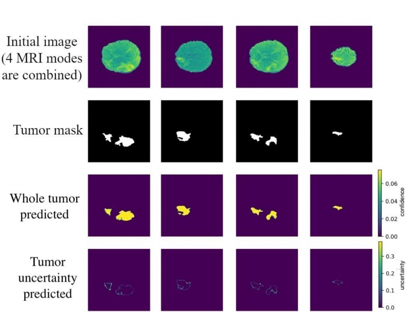
Tell us more about your project. What kind of feedback did you receive? 

A year ago we sent our work to the conference of The Medical Image Computing and Computer Assisted Intervention Society (MICCAI), but we were refused a publication because another group of researchers came up with the same method about the same time. And we didn’t even know, our projects came out only a couple of months apart. 

That’s why this year we decided to rework our article and focus not on the new method but on its applications in medical data. We sent the article to The Conference on Uncertainty in Artificial Intelligence (UAI), the world’s main conference on AI, where it was accepted for the workshop on applied Bayesian modeling. As I was presenting at the conference, I received an email from  MICCAI: they had accepted our article, but for that we had to come up with a whole new way for measuring uncertainty. 

What changed in the research method?

Over the course of this year we experimented with various methods similar to dropout that weren’t used to measure uncertainty before. Once I suggested taking NASNet, Google’s most precise network for image processing, as our basis.  

A regularization technique called Scheduled DropPath was developed specifically for it. It is similar to dropout, but its creator suggested excluding complete paths in convolution units with a growing dropout probability.  

As it’s a rather efficient network, we decided to apply it to tumor detection. Then, we used Scheduled DropPath in the Monte Carlo fashion to measure uncertainty. We got an improvement of 0.8%, which is cool but might seem as random for those who don’t know the details. So we decided to go even further.

Both DropPath and dropout have a fixed dropout probability. Instead, we decided to look for the best probability, the one that would ensure the highest detection accuracy. We could search for it manually, or we could optimize the process, just like neural networks do during training. That means that dropout probabilities are now also trainable. This method is called concrete dropout. We applied it in our project and developed a new method that we called Monte Carlo Concrete DropPath. 

Using this new distribution we raised the accuracy even more and improved the calibration of our model. It can now measure uncertainty better, as the calibration became twice as good, while the accuracy rose 3%. This method is better and more accurate than its analogs. The related articles will be published in CEUR Workshop Proceedings and Lecture Notes in Computer Science.

How can the method you developed be applied in practice? 

Speaking of the task of measuring uncertainty, we didn’t work on implementing, that’s what our collaborators are responsible for. But the better the model, the more accurate its predictions on brain tumors. The visualized uncertainty that we can predict using Bayesian methods helps to see where the model isn’t confident. 

This is a universally applicable method. For instance, I am using it in my thesis on detecting allergenic pollen images. I developed a web service based on deep neural networks, which will notify its users when allergens appear in their city.